Electrical Resistivity Monitoring Primer

Data processing

Inversion concept

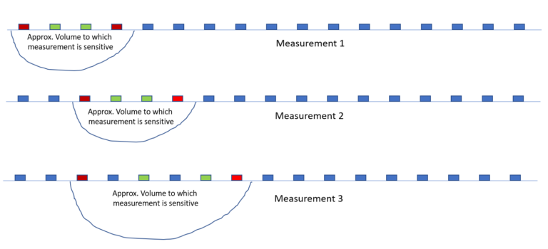
As mentioned in the data acquisition section an electrical resistivity survey contains hundreds to thousands of measurements. taken with different combinations of electrodes. Each of these measurements is sensitive to a different part of the subsurface.

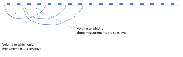
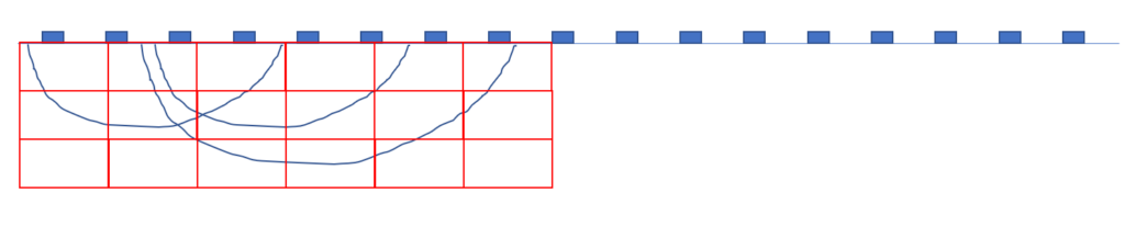
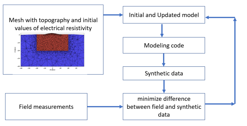
We want to translate these measurements into a volumetric distribution of resistivity values of the subsurface. This is done through a process known as inversion. In order to understand this process, it is helpful to consider the cartoons below which explain the concept underneath this process.

The first cartoon shows three measurements. In each measurement we have the current electrodes in red and the potential electrodes in green.

For each of these three measurements (of course, in practice we will have many more), there is a volume to which this measurement is sensitive. As shown below, these volumes overlap.

We can now create a grid (for example the one below, where we have 18 grid blocks), and assign resistivity values to each of the blocks. We can calculate the effect of each grid block on each measurement numerically. By changing the values of the resistivity values in each block we can find a combination which gives the best fit between the observed and synthetic data.

Inversion in practice

In practice we use a numerical code to perform inversion. A number of codes (both open source and commercial codes) are available for this (see here for a list). The steps involved in this are shown schematically below. The numerical code starts with an initial distribution of resistivities. This distribution is given on a mesh which also includes the topography. In this mesh every cell has a resistivity value. This is the so called initial model. In addition to this we have the observed (measured) data. The numerical code now uses an algorithm to calculate synthetic data with the same geometry as our field measurements. We know compare these data. Our objective in inversion is to minimize their difference, and we do this by updating the resistivity values on the mesh and repeating this process unless we achieve our target difference. This then gives us our subsurface resistivity distribution. Note that this description is simplified. For a more in depth discussion about inversion see e.g. this website from the University of British Columbia.

Why do resistivity models look smooth?

One important concept to understand is the reason why resistivity models typically look smooth (while in general the earth does not have a smooth distribution of physical properties). The reason behind this is that in inversion we have a quandary: given the fact that inversion is non unique: an infinite set of conductivity models exist which fit the data (see the classical paper by deGroot-Hedlin and Constable from 1990), and the question is thus how we decide which one of these models to use. A very common answer is to use a smooth model, which we do by applying a smoothness constraint in our numerical solution (essentially penalizing large local variations and oscillations in resistivity).